(this is a continuation from Part 1)

Select the shapefile (and re-project if necessary)

A description of the structure of ESRI shapefiles and their treatment by the gdal library are covered here.

Let’s read the actual shapefiles. The rgdal package reads them into a spatial object: a SpatialPolygonsDataFrame, to recognise their dual nature (polygons + data).

> ewAll <- readOGR(dsn=dns, layer="LSOA_2011_EW_BFC_V2",  stringsAsFactors=FALSE)
OGR data source with driver: ESRI Shapefile 
Source: "/Users/e/Dropbox/dev/DevLib/MyGISLib/Lower_layer_super_output_areas_(E+W)_2011_Boundaries_(Full_Clipped)_V2", layer: "LSOA_2011_EW_BFC_V2"
with 34753 features
It has 3 fields
> proj4string(ewAll)
[1] "+proj=tmerc +lat_0=49 +lon_0=-2 +k=0.9996012717 +x_0=400000 +y_0=-100000 +datum=OSGB36 +units=m +no_defs +ellps=airy +towgs84=446.448,-125.157,542.060,0.1502,0.2470,0.8421,-20.4894"
# It is helpful understand the class of the ewAll object
> class(ewAll)
  [1] "SpatialPolygonsDataFrame"
  attr(,"package")
  [1] "sp"

I mentioned in Part 1 that the shapefiles from ONS (and Ordnance Survey) follow OSGB36. Here proj4string gives additional information (I suspect this function comes from proj4 rather than gdal: maybe this explains the difference). The shapefile already includes transformations to a global datum, specified by +towgs84. these consitute the famous seven point Helmert transformation. If they are absent the results will be sub-optimal (believe me!).

In Part 1 we have already encountered the “data” part of the shapefile:

Number of fields: 3 
    Name      type length typeName
1  LSOA11CD    4      9   String
2  LSOA11NM    4    254   String
3 LSOA11NMW    4    254   String

As the ONS documentation clarifies, the LSOA for the 2011 census come in:
- Code names of 9 characters
- Names of up to 254 characters
- Welsh names (for Welsh locations) of up to 254 characters

Let’s see what sort of data we have inside the shapefiles.

> head(ewAll@data)
   LSOA11CD                  LSOA11NM                 LSOA11NMW
0 E01000001       City of London 001A       City of London 001A
1 E01000002       City of London 001B       City of London 001B
2 E01000003       City of London 001C       City of London 001C
3 E01000005       City of London 001E       City of London 001E
4 E01000006 Barking and Dagenham 016A Barking and Dagenham 016A
5 E01000007 Barking and Dagenham 015A Barking and Dagenham 015A

Therefore the plan of attack is clear:
- If we need to subset the shapefile, we should be able to find the area(s) of interest searching the extended names.
- If we will need to link data to the shape we will use the code names (much more about this later).
- With respect to the Welsh, we will delete LSOA11NMW (we could just ignore it, but is going to take space for more relevant information).

As the Data Dive I’ve attended was about Leeds, I will select the shapefiles referring to Leeds.

>leedsST <- ewAll[grepl( "Leeds", ewAll$LSOA11NM),]
> nrow(leedsST)
[1] 482
#
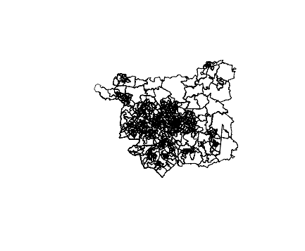
plot(leedsST)

In this case I know that all the LSOA shapes in Leeds have “Leeds” in the name. In some other case it will be more complex, but often is possible to find lookup tables to ease the task.
This gives us 482 polygons for all the Leeds area. As the average population ofr a LSOA is 1,500 inhabitants, a quick check (482*1,500) will tell us that the order of magnitude is correct. Good!

We can now plot the shapefile. Plotting the whole E+W shapefile would have been too much for RStudio, my IDE of choice (and even tools like QGIS struggle a bit for the sheer number of polygons to display).

Now we will change the projection, moving from OSGB36 to WSG84.

leedsCoor <- CRS("+proj=longlat +datum=WGS84")
newLeedsShape <- spTransform(leedsST, leedsCoor)

We could re-plot the shapefiles, but probably at this stage we wouldn’t notice a major difference.

Simplify the shapefile and save it to geojson

This step is very simple. Basically a polygon contains numerous nodes, i.e. points: every nook and cranny of the area of reference is detailed. This is too much detail for a choropleth. The size of the Leeds shapefile we have obtained is around 16Mb. This would make it difficult to show our choropleth on a mobile phone.

The solution is simple: it is possible to simplify the polygons in a number of ways, for example reducing the number of nodes. We will use the well established Ramer–Douglas–Peucker algorithm (RDP) to reduce the number of points in a curve that is approximated by a series of points (please note that I’ll mention topojson later in another part of the tutorial).

We need to be careful though: too much simplification and the polygons will start to “open up”: basically they will not appear attached to each other any more and holes will start to manifest. This is where it is convenient to use tools like QGIS to visually play with the best tolerance coefficient for the simplification.
This time I will be satisfied with a reduction to ~10% of the original size.
The simplification uses gSimplify from the rgdal package.

# gSimplify strips the data portion away - it needs to be saved first
>df <- newLeedsShape@data
#
>newLeedsSimp <- gSimplify(newLeedsShape, 0.00005, topologyPreserve=TRUE)
# now we can recombine the two portions of the SpatialPolygonsDataFrame
>newLeedsSimpShape <- SpatialPolygonsDataFrame(newLeedsSimp,data=df)
# eventually we can save the file to geojson
>writeOGR(newLeedsSimpShape,'./data/newLeedsSimp.geojson','newLeedsSimpShape', driver='GeoJSON',check_exists = FALSE)

The original shapefile has been seriously simplified and re-projected. What if we have made some mistake along the way?

A very simple, but very useful trick we can use to check on our geojson is to load it in a gist in github.

Github will render the shapefile over a zoomable map of the area (currently based on openstreetmap - see below): we can see directly the quality of what we have done so far.

Another interesting characteristic of our map is that clicking on a polygon will display its Code Name and Name. We will come back to exploit this feature later.

The method of using github is great and in my experience a fundamental part of the process, allowing to spot projection errors etc. before going too far ahead.

A side note

During the preparation of this simple tutorial I’ve discovered a few interesting things I had forgotten or I didn’t know.

• geojson standard is actually based on a WGS84 projection. If you want to be really specific, “urn:ogc:def:crs:OGC:1.3:CRS84”. This info is in the beginning of the geojson file as CRS.
• rgdal / gdal automatically re-project the shapefiles when saving to geojson if it is not already in the right CRS: you could possibly save the re-projection step if you save to geojson.
• Github renders in their gists only geojson (and topojson). One of the implications is that github supports only urn:ogc:def:crs:OGC:1.3:CRS84 (e.g. WGS84).
• Github uses a openstreetmap (currently the mainstream open source map) layer to render geojson in their gists. .
• As the Ordnance Survey site puts it, it is a myth to believe that it is possible to re-project exactly from one CRS to another with a simple algorithm: you are bound to have projection errors. Especially on a large scale it would be good to have an idea of where you are going to have the largest errors - and how big is going to be. Even a “complex” one like the seven point Helmert transformation gives some residual errors.

This concludes Part 2 of this series. Next part will address the data preparation.